bupaR Docs | Filter case

---

Case filters

library(bupaverse)

Activity presence

Usefilter_activity_presence() to select cases that contain a specific activity, for instance an X-Ray scan. The function returns a log object. For the illustration purposes traces() is also used.

patients %>%
    filter_activity_presence("X-Ray") %>%
    traces()

## # A tibble: 3 × 3
##   trace                                    absolute_frequency relative_frequency
##   <chr>                                                 <int>              <dbl>
## 1 Registration,Triage and Assessment,X-Ra…                258            0.989  
## 2 Registration,Triage and Assessment,X-Ray                  2            0.00766
## 3 Registration,Triage and Assessment,X-Ra…                  1            0.00383

Or that don’t have a specific activity, using reserve = TRUE.

patients %>%
    filter_activity_presence("X-Ray", reverse = TRUE) %>%
    traces()

## # A tibble: 4 × 3
##   trace                                    absolute_frequency relative_frequency
##   <chr>                                                 <int>              <dbl>
## 1 Registration,Triage and Assessment,Bloo…                234            0.979  
## 2 Registration,Triage and Assessment,Bloo…                  2            0.00837
## 3 Registration,Triage and Assessment                        2            0.00837
## 4 Registration,Triage and Assessment,Bloo…                  1            0.00418

We can also specify more than one activity. In this case, the method argument can be configured as follows:

• “all” means that all the specified activity labels must be present for a case to be selected.
• “none” means that they are not allowed to be present.
• “one_of” means that at least one of them must be present.
• “exact” means that all of these activities have to be present (although multiple times and in random orderings), while no others are allowed.
• “only” means that only (a set of) these activities are allowed to be present, and no others.

Below an illustration of these different options for the activities Create Fine and Payment from traffic_fines. Note that the unfiltered dataset has 44 distinct traces.

All

27 traces have both activities.

traffic_fines %>%
    filter_activity_presence(c("Create Fine", "Payment"), method = "all")  %>%
    traces()

## # A tibble: 27 × 3
##    trace                                   absolute_frequency relative_frequency
##    <chr>                                                <int>              <dbl>
##  1 Create Fine,Payment                                   3428            0.741  
##  2 Create Fine,Send Fine,Insert Fine Noti…                758            0.164  
##  3 Create Fine,Send Fine,Insert Fine Noti…                250            0.0540 
##  4 Create Fine,Send Fine,Insert Fine Noti…                 78            0.0169 
##  5 Create Fine,Send Fine,Payment                           37            0.00800
##  6 Create Fine,Send Fine,Insert Fine Noti…                 13            0.00281
##  7 Create Fine,Send Fine,Insert Fine Noti…                  9            0.00195
##  8 Create Fine,Send Fine,Insert Fine Noti…                  8            0.00173
##  9 Create Fine,Send Fine,Insert Fine Noti…                  7            0.00151
## 10 Create Fine,Send Fine,Insert Fine Noti…                  5            0.00108
## # ℹ 17 more rows

None

No traces exist that have none of these activities.

traffic_fines %>%
    filter_activity_presence(c("Create Fine", "Payment"), method = "none")  %>%
    traces()

## [1] trace              absolute_frequency relative_frequency
## <0 rows> (or 0-length row.names)

One of

All 44 traces have at least one of these activities.

traffic_fines %>%
    filter_activity_presence(c("Create Fine", "Payment"), method = "one_of")  %>%
    traces()

## # A tibble: 44 × 3
##    trace                                   absolute_frequency relative_frequency
##    <chr>                                                <int>              <dbl>
##  1 Create Fine,Payment                                   3428             0.343 
##  2 Create Fine,Send Fine,Insert Fine Noti…               3273             0.327 
##  3 Create Fine,Send Fine                                 1890             0.189 
##  4 Create Fine,Send Fine,Insert Fine Noti…                758             0.0758
##  5 Create Fine,Send Fine,Insert Fine Noti…                250             0.025 
##  6 Create Fine,Send Fine,Insert Fine Noti…                151             0.0151
##  7 Create Fine,Send Fine,Insert Fine Noti…                 78             0.0078
##  8 Create Fine,Send Fine,Payment                           37             0.0037
##  9 Create Fine,Send Fine,Insert Fine Noti…                 24             0.0024
## 10 Create Fine,Send Fine,Insert Fine Noti…                 13             0.0013
## # ℹ 34 more rows

Exact

Only 2 traces consist of exactly these activities.

traffic_fines %>%
    filter_activity_presence(c("Create Fine", "Payment"), method = "exact")  %>%
    traces()

## # A tibble: 2 × 3
##   trace                       absolute_frequency relative_frequency
##   <chr>                                    <int>              <dbl>
## 1 Create Fine,Payment                       3428           0.999   
## 2 Create Fine,Payment,Payment                  2           0.000583

Only

And the same 2 traces have only these activities.

traffic_fines %>%
    filter_activity_presence(c("Create Fine", "Payment"), method = "only")  %>%
    traces()

## # A tibble: 2 × 3
##   trace                       absolute_frequency relative_frequency
##   <chr>                                    <int>              <dbl>
## 1 Create Fine,Payment                       3428           0.999   
## 2 Create Fine,Payment,Payment                  2           0.000583

Note that when one of the specified activities cannot be found in the log, you will get a warning about this. However, filter_activity_presence() will proceed with the specified list in any case. The result below shows that no trace has the activity “Create Fines”.

traffic_fines %>%
    filter_activity_presence(c("Create Fines"), method = "none")  %>%
    traces()

## Warning in filter_activity_presence(., c("Create Fines"), method = "none"): 1 specified activity in `activities` not found in `log`.
## ! Activity not found and ignored: "Create Fines".

## [1] trace              absolute_frequency relative_frequency
## <0 rows> (or 0-length row.names)

Case

filter_case() can be used to filter cases based on their identifier. It returns the same log object containing events with the specified cases.

traffic_fines %>%
    filter_case(cases = c("A1","A2"))

## # Log of 4 events consisting of:
## 1 trace 
## 2 cases 
## 4 instances of 2 activities 
## 2 resources 
## Events occurred from 2006-07-24 until 2006-12-05 
##  
## # Variables were mapped as follows:
## Case identifier:     case_id 
## Activity identifier:     activity 
## Resource identifier:     resource 
## Activity instance identifier:    activity_instance_id 
## Timestamp:           timestamp 
## Lifecycle transition:        lifecycle 
## 
## # A tibble: 4 × 18
##   case_id activity    lifecycle resource timestamp           amount article
##   <chr>   <fct>       <fct>     <fct>    <dttm>              <chr>    <dbl>
## 1 A1      Create Fine complete  561      2006-07-24 00:00:00 35.0       157
## 2 A1      Send Fine   complete  <NA>     2006-12-05 00:00:00 <NA>        NA
## 3 A2      Create Fine complete  561      2006-07-24 00:00:00 35.0       157
## 4 A2      Send Fine   complete  <NA>     2006-12-05 00:00:00 <NA>        NA
## # ℹ 11 more variables: dismissal <chr>, expense <chr>, lastsent <chr>,
## #   matricola <dbl>, notificationtype <chr>, paymentamount <dbl>, points <dbl>,
## #   totalpaymentamount <chr>, vehicleclass <chr>, activity_instance_id <chr>,
## #   .order <int>

The selection can be reversed with reverse = TRUE.

traffic_fines %>%
    filter_case(cases = c("A1","A2"), reverse = TRUE)

## # Log of 34720 events consisting of:
## 44 traces 
## 9998 cases 
## 34720 instances of 11 activities 
## 16 resources 
## Events occurred from 2006-06-17 until 2012-03-26 
##  
## # Variables were mapped as follows:
## Case identifier:     case_id 
## Activity identifier:     activity 
## Resource identifier:     resource 
## Activity instance identifier:    activity_instance_id 
## Timestamp:           timestamp 
## Lifecycle transition:        lifecycle 
## 
## # A tibble: 34,720 × 18
##    case_id activity        lifecycle resource timestamp           amount article
##    <chr>   <fct>           <fct>     <fct>    <dttm>              <chr>    <dbl>
##  1 A100    Create Fine     complete  561      2006-08-02 00:00:00 35.0       157
##  2 A100    Send Fine       complete  <NA>     2006-12-12 00:00:00 <NA>        NA
##  3 A100    Insert Fine No… complete  <NA>     2007-01-15 00:00:00 <NA>        NA
##  4 A100    Add penalty     complete  <NA>     2007-03-16 00:00:00 71.5        NA
##  5 A100    Send for Credi… complete  <NA>     2009-03-30 00:00:00 <NA>        NA
##  6 A10000  Create Fine     complete  561      2007-03-09 00:00:00 36.0       157
##  7 A10000  Send Fine       complete  <NA>     2007-07-17 00:00:00 <NA>        NA
##  8 A10000  Insert Fine No… complete  <NA>     2007-08-02 00:00:00 <NA>        NA
##  9 A10000  Add penalty     complete  <NA>     2007-10-01 00:00:00 74.0        NA
## 10 A10000  Payment         complete  <NA>     2008-09-09 00:00:00 <NA>        NA
## # ℹ 34,710 more rows
## # ℹ 11 more variables: dismissal <chr>, expense <chr>, lastsent <chr>,
## #   matricola <dbl>, notificationtype <chr>, paymentamount <dbl>, points <dbl>,
## #   totalpaymentamount <chr>, vehicleclass <chr>, activity_instance_id <chr>,
## #   .order <int>

Case Condition

filter_case_condition() can be used to select cases for which a condition holds. This condition can be related to any of the variables in the log.

For example, select all cases where resource 561 is involved.

traffic_fines %>%
    filter_case_condition(resource == 561)

## # Log of 3333 events consisting of:
## 17 traces 
## 1002 cases 
## 3333 instances of 11 activities 
## 3 resources 
## Events occurred from 2006-07-01 until 2012-03-26 
##  
## # Variables were mapped as follows:
## Case identifier:     case_id 
## Activity identifier:     activity 
## Resource identifier:     resource 
## Activity instance identifier:    activity_instance_id 
## Timestamp:           timestamp 
## Lifecycle transition:        lifecycle 
## 
## # A tibble: 3,333 × 18
##    case_id activity        lifecycle resource timestamp           amount article
##    <chr>   <fct>           <fct>     <fct>    <dttm>              <chr>    <dbl>
##  1 A1      Create Fine     complete  561      2006-07-24 00:00:00 35.0       157
##  2 A1      Send Fine       complete  <NA>     2006-12-05 00:00:00 <NA>        NA
##  3 A100    Create Fine     complete  561      2006-08-02 00:00:00 35.0       157
##  4 A100    Send Fine       complete  <NA>     2006-12-12 00:00:00 <NA>        NA
##  5 A100    Insert Fine No… complete  <NA>     2007-01-15 00:00:00 <NA>        NA
##  6 A100    Add penalty     complete  <NA>     2007-03-16 00:00:00 71.5        NA
##  7 A100    Send for Credi… complete  <NA>     2009-03-30 00:00:00 <NA>        NA
##  8 A10000  Create Fine     complete  561      2007-03-09 00:00:00 36.0       157
##  9 A10000  Send Fine       complete  <NA>     2007-07-17 00:00:00 <NA>        NA
## 10 A10000  Insert Fine No… complete  <NA>     2007-08-02 00:00:00 <NA>        NA
## # ℹ 3,323 more rows
## # ℹ 11 more variables: dismissal <chr>, expense <chr>, lastsent <chr>,
## #   matricola <dbl>, notificationtype <chr>, paymentamount <dbl>, points <dbl>,
## #   totalpaymentamount <chr>, vehicleclass <chr>, activity_instance_id <chr>,
## #   .order <int>

Note that multiple conditions can be combined using the symbols | (or) and & (and). For example, let’s select all cases where resource 557 is involved, and the points are more than 0.

traffic_fines %>%
    filter_case_condition(resource == 557 & points > 0)

## # Log of 10 events consisting of:
## 1 trace 
## 2 cases 
## 10 instances of 5 activities 
## 2 resources 
## Events occurred from 2007-03-12 until 2010-10-15 
##  
## # Variables were mapped as follows:
## Case identifier:     case_id 
## Activity identifier:     activity 
## Resource identifier:     resource 
## Activity instance identifier:    activity_instance_id 
## Timestamp:           timestamp 
## Lifecycle transition:        lifecycle 
## 
## # A tibble: 10 × 18
##    case_id activity        lifecycle resource timestamp           amount article
##    <chr>   <fct>           <fct>     <fct>    <dttm>              <chr>    <dbl>
##  1 A10141  Create Fine     complete  557      2007-03-12 00:00:00 74.0       158
##  2 A10141  Send Fine       complete  <NA>     2007-07-17 00:00:00 <NA>        NA
##  3 A10141  Insert Fine No… complete  <NA>     2007-07-26 00:00:00 <NA>        NA
##  4 A10141  Add penalty     complete  <NA>     2007-09-24 00:00:00 148.0       NA
##  5 A10141  Send for Credi… complete  <NA>     2009-03-30 00:00:00 <NA>        NA
##  6 A25817  Create Fine     complete  557      2008-03-01 00:00:00 74.0       158
##  7 A25817  Send Fine       complete  <NA>     2008-06-04 00:00:00 <NA>        NA
##  8 A25817  Insert Fine No… complete  <NA>     2008-06-09 00:00:00 <NA>        NA
##  9 A25817  Add penalty     complete  <NA>     2008-08-08 00:00:00 148.0       NA
## 10 A25817  Send for Credi… complete  <NA>     2010-10-15 00:00:00 <NA>        NA
## # ℹ 11 more variables: dismissal <chr>, expense <chr>, lastsent <chr>,
## #   matricola <dbl>, notificationtype <chr>, paymentamount <dbl>, points <dbl>,
## #   totalpaymentamount <chr>, vehicleclass <chr>, activity_instance_id <chr>,
## #   .order <int>

Conditions can be reversed using ! or the reverse = TRUE argument. The following to commands are equivalent.

traffic_fines %>%
    filter_case_condition(!(resource == 557 & points > 0))

## # Log of 34714 events consisting of:
## 44 traces 
## 9998 cases 
## 34714 instances of 11 activities 
## 16 resources 
## Events occurred from 2006-06-17 until 2012-03-26 
##  
## # Variables were mapped as follows:
## Case identifier:     case_id 
## Activity identifier:     activity 
## Resource identifier:     resource 
## Activity instance identifier:    activity_instance_id 
## Timestamp:           timestamp 
## Lifecycle transition:        lifecycle 
## 
## # A tibble: 34,714 × 18
##    case_id activity        lifecycle resource timestamp           amount article
##    <chr>   <fct>           <fct>     <fct>    <dttm>              <chr>    <dbl>
##  1 A1      Create Fine     complete  561      2006-07-24 00:00:00 35.0       157
##  2 A1      Send Fine       complete  <NA>     2006-12-05 00:00:00 <NA>        NA
##  3 A100    Create Fine     complete  561      2006-08-02 00:00:00 35.0       157
##  4 A100    Send Fine       complete  <NA>     2006-12-12 00:00:00 <NA>        NA
##  5 A100    Insert Fine No… complete  <NA>     2007-01-15 00:00:00 <NA>        NA
##  6 A100    Add penalty     complete  <NA>     2007-03-16 00:00:00 71.5        NA
##  7 A100    Send for Credi… complete  <NA>     2009-03-30 00:00:00 <NA>        NA
##  8 A10000  Create Fine     complete  561      2007-03-09 00:00:00 36.0       157
##  9 A10000  Send Fine       complete  <NA>     2007-07-17 00:00:00 <NA>        NA
## 10 A10000  Insert Fine No… complete  <NA>     2007-08-02 00:00:00 <NA>        NA
## # ℹ 34,704 more rows
## # ℹ 11 more variables: dismissal <chr>, expense <chr>, lastsent <chr>,
## #   matricola <dbl>, notificationtype <chr>, paymentamount <dbl>, points <dbl>,
## #   totalpaymentamount <chr>, vehicleclass <chr>, activity_instance_id <chr>,
## #   .order <int>

traffic_fines %>%
    filter_case_condition(resource == 557 & points > 0, reverse = TRUE)

## # Log of 34714 events consisting of:
## 44 traces 
## 9998 cases 
## 34714 instances of 11 activities 
## 16 resources 
## Events occurred from 2006-06-17 until 2012-03-26 
##  
## # Variables were mapped as follows:
## Case identifier:     case_id 
## Activity identifier:     activity 
## Resource identifier:     resource 
## Activity instance identifier:    activity_instance_id 
## Timestamp:           timestamp 
## Lifecycle transition:        lifecycle 
## 
## # A tibble: 34,714 × 18
##    case_id activity        lifecycle resource timestamp           amount article
##    <chr>   <fct>           <fct>     <fct>    <dttm>              <chr>    <dbl>
##  1 A1      Create Fine     complete  561      2006-07-24 00:00:00 35.0       157
##  2 A1      Send Fine       complete  <NA>     2006-12-05 00:00:00 <NA>        NA
##  3 A100    Create Fine     complete  561      2006-08-02 00:00:00 35.0       157
##  4 A100    Send Fine       complete  <NA>     2006-12-12 00:00:00 <NA>        NA
##  5 A100    Insert Fine No… complete  <NA>     2007-01-15 00:00:00 <NA>        NA
##  6 A100    Add penalty     complete  <NA>     2007-03-16 00:00:00 71.5        NA
##  7 A100    Send for Credi… complete  <NA>     2009-03-30 00:00:00 <NA>        NA
##  8 A10000  Create Fine     complete  561      2007-03-09 00:00:00 36.0       157
##  9 A10000  Send Fine       complete  <NA>     2007-07-17 00:00:00 <NA>        NA
## 10 A10000  Insert Fine No… complete  <NA>     2007-08-02 00:00:00 <NA>        NA
## # ℹ 34,704 more rows
## # ℹ 11 more variables: dismissal <chr>, expense <chr>, lastsent <chr>,
## #   matricola <dbl>, notificationtype <chr>, paymentamount <dbl>, points <dbl>,
## #   totalpaymentamount <chr>, vehicleclass <chr>, activity_instance_id <chr>,
## #   .order <int>

Endpoints

filter_endpoints() allows to select cases with a specific start and/or end activity. In case of the patients data set, all cases start with “Registration”. Filtering cases that don’t start with Registration (reverse = TRUE) gives an empty log.

patients %>%
    filter_endpoints(start_activities = "Registration", reverse = TRUE)

## EMPTY EVENT LOG
## # A tibble: 0 × 7
## # ℹ 7 variables: handling <fct>, patient <chr>, employee <fct>,
## #   handling_id <chr>, registration_type <fct>, time <dttm>, .order <int>

If we are interested to see the “completed” cases, those that start with Registration and end we “Check-out”, we can apply the following filter. Here process_map() is used for the illustration purposes.

patients %>%
    filter_endpoints(start_activities = "Registration", end_activities = "Check-out") %>%
    process_map()

Endpoints Condition

filter_endpoints_condition() allows to select cases by applying conditions to the start and/or end activity instance. For example. We can use it to replace the filter_endpoints() from above, using conditions on the handling variable.

patients %>%
    filter_endpoints_condition(start_condition = handling  == "Registration", end_condition = handling  == "Check-out")

## # Log of 5388 events consisting of:
## 2 traces 
## 492 cases 
## 2694 instances of 7 activities 
## 7 resources 
## Events occurred from 2017-01-02 11:41:53 until 2018-05-03 03:34:55 
##  
## # Variables were mapped as follows:
## Case identifier:     patient 
## Activity identifier:     handling 
## Resource identifier:     employee 
## Activity instance identifier:    handling_id 
## Timestamp:           time 
## Lifecycle transition:        registration_type 
## 
## # A tibble: 5,388 × 7
##    handling   patient employee handling_id registration_type time               
##    <fct>      <chr>   <fct>    <chr>       <fct>             <dttm>             
##  1 Registrat… 1       r1       1           start             2017-01-02 11:41:53
##  2 Registrat… 2       r1       2           start             2017-01-02 11:41:53
##  3 Registrat… 3       r1       3           start             2017-01-04 01:34:05
##  4 Registrat… 4       r1       4           start             2017-01-04 01:34:04
##  5 Registrat… 5       r1       5           start             2017-01-04 16:07:47
##  6 Registrat… 6       r1       6           start             2017-01-04 16:07:47
##  7 Registrat… 7       r1       7           start             2017-01-05 04:56:11
##  8 Registrat… 8       r1       8           start             2017-01-05 04:56:11
##  9 Registrat… 9       r1       9           start             2017-01-06 05:58:54
## 10 Registrat… 10      r1       10          start             2017-01-06 05:58:54
## # ℹ 5,378 more rows
## # ℹ 1 more variable: .order <int>

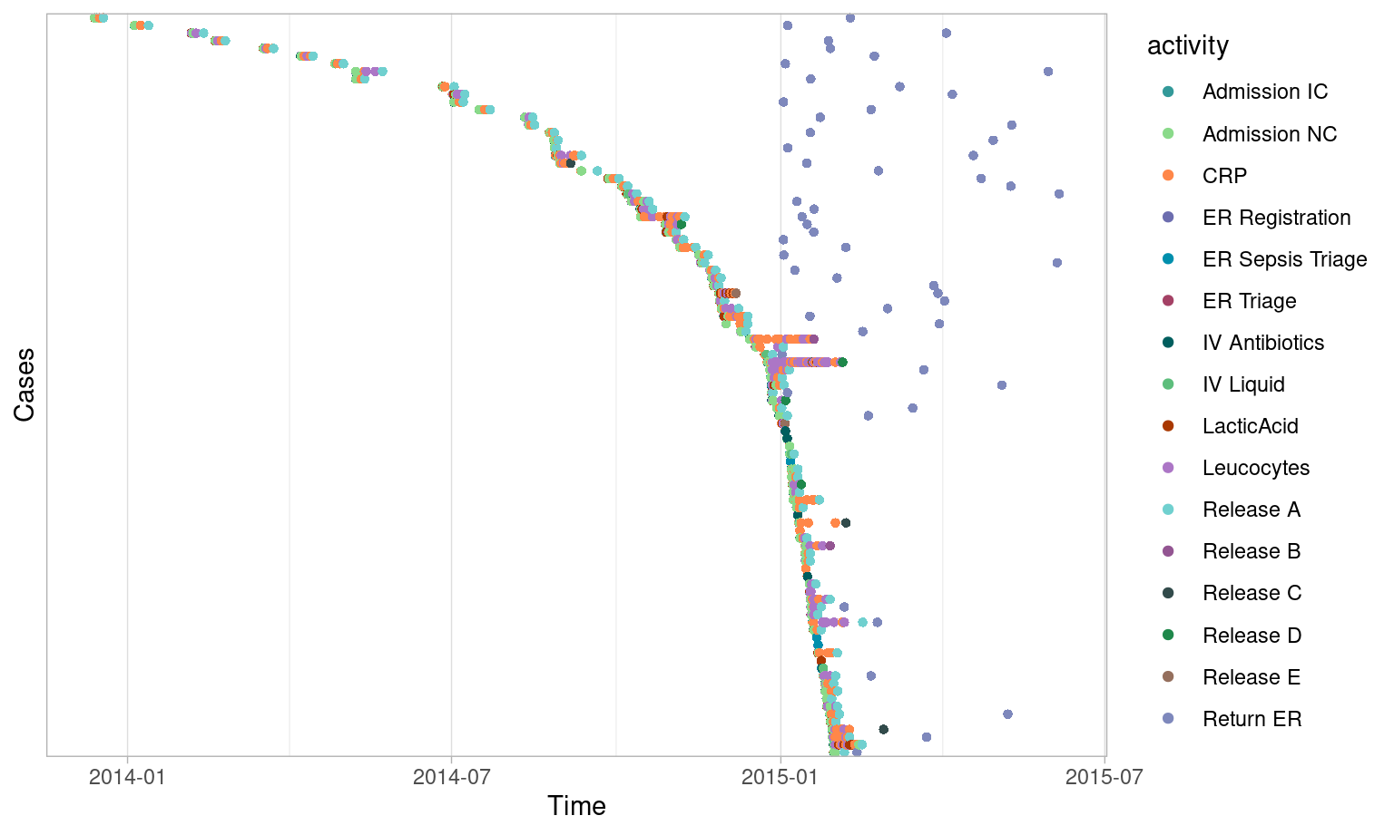
Naturally, both conditions can use any of the available variables. The following selects all cases that started between midnight and 6am. Note that no condition is applied on the end activity instance using the end_condition = TRUE specification. We use dotted_chart("relative_day") to plot a graph where, each activity instance is displayed with a dot. The x-axis refers to the time aspect (here a relative time difference since the first case on x-axis), while the y-axis refers to cases.

patients %>%
    filter_endpoints_condition(start_condition = lubridate::hour(time) < 6, end_condition = TRUE) %>%
    dotted_chart("relative_day")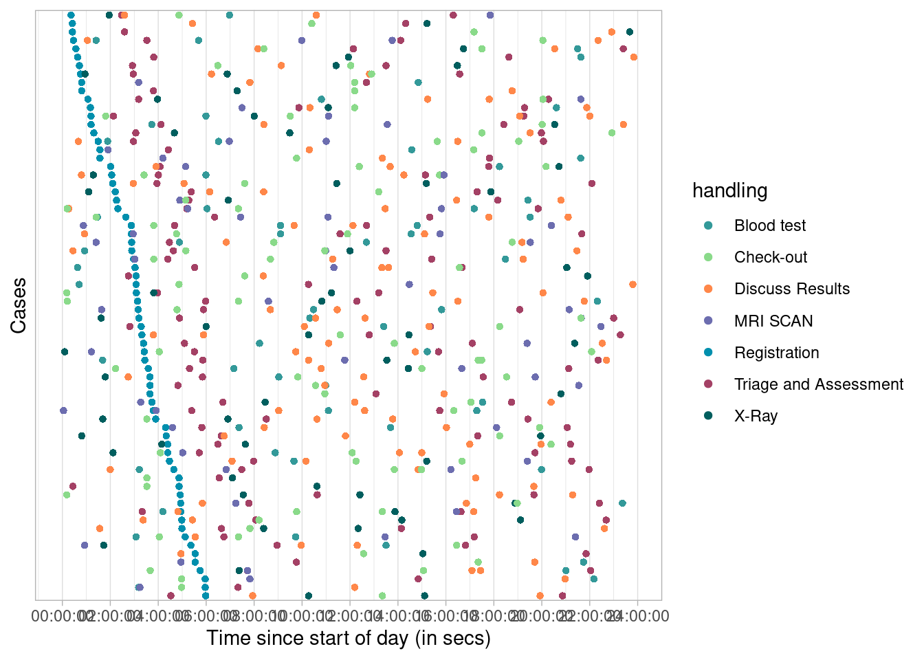

Flow Time

filter_flow_time() can be used to select cases in which a specific directly-follows flow (from > to) happens within a specific time duration interval.

For example, we can select the fines from traffic_fines in which the creation is followed by the payment within 4 weeks.

traffic_fines %>%
    filter_flow_time(from = "Create Fine", to = "Payment", interval = c(0,4), units = "weeks")

## # Log of 6303 events consisting of:
## 5 traces 
## 3143 cases 
## 6303 instances of 6 activities 
## 15 resources 
## Events occurred from 2006-07-26 until 2010-10-15 
##  
## # Variables were mapped as follows:
## Case identifier:     case_id 
## Activity identifier:     activity 
## Resource identifier:     resource 
## Activity instance identifier:    activity_instance_id 
## Timestamp:           timestamp 
## Lifecycle transition:        lifecycle 
## 
## # A tibble: 6,303 × 18
##    case_id activity    lifecycle resource timestamp           amount article
##    <chr>   <fct>       <fct>     <fct>    <dttm>              <chr>    <dbl>
##  1 A10005  Create Fine complete  537      2007-03-20 00:00:00 36.0       157
##  2 A10005  Payment     complete  <NA>     2007-03-21 00:00:00 <NA>        NA
##  3 A10007  Create Fine complete  537      2007-03-20 00:00:00 36.0       157
##  4 A10007  Payment     complete  <NA>     2007-03-23 00:00:00 <NA>        NA
##  5 A10022  Create Fine complete  537      2007-03-22 00:00:00 22.0         7
##  6 A10022  Payment     complete  <NA>     2007-03-28 00:00:00 <NA>        NA
##  7 A10024  Create Fine complete  537      2007-03-22 00:00:00 36.0       157
##  8 A10024  Payment     complete  <NA>     2007-03-26 00:00:00 <NA>        NA
##  9 A10029  Create Fine complete  537      2007-03-22 00:00:00 36.0       157
## 10 A10029  Payment     complete  <NA>     2007-04-10 00:00:00 <NA>        NA
## # ℹ 6,293 more rows
## # ℹ 11 more variables: dismissal <chr>, expense <chr>, lastsent <chr>,
## #   matricola <dbl>, notificationtype <chr>, paymentamount <dbl>, points <dbl>,
## #   totalpaymentamount <chr>, vehicleclass <chr>, activity_instance_id <chr>,
## #   .order <int>

The interval can be defined as half-open using NA for the first or second element. Below select cases where payment is followed after 4 weeks.

traffic_fines %>%
    filter_flow_time(from = "Create Fine", to = "Payment", interval = c(4, NA), units = "weeks")

## # Log of 646 events consisting of:
## 6 traces 
## 312 cases 
## 646 instances of 6 activities 
## 15 resources 
## Events occurred from 2006-06-17 until 2009-03-30 
##  
## # Variables were mapped as follows:
## Case identifier:     case_id 
## Activity identifier:     activity 
## Resource identifier:     resource 
## Activity instance identifier:    activity_instance_id 
## Timestamp:           timestamp 
## Lifecycle transition:        lifecycle 
## 
## # A tibble: 646 × 18
##    case_id activity    lifecycle resource timestamp           amount article
##    <chr>   <fct>       <fct>     <fct>    <dttm>              <chr>    <dbl>
##  1 A10059  Create Fine complete  541      2007-03-08 00:00:00 36.0       157
##  2 A10059  Payment     complete  <NA>     2007-04-18 00:00:00 <NA>        NA
##  3 A1006   Create Fine complete  550      2006-08-08 00:00:00 21.0         7
##  4 A1006   Payment     complete  <NA>     2006-09-12 00:00:00 <NA>        NA
##  5 A10157  Create Fine complete  558      2007-03-06 00:00:00 36.0       157
##  6 A10157  Payment     complete  <NA>     2007-04-13 00:00:00 <NA>        NA
##  7 A10221  Create Fine complete  559      2007-03-09 00:00:00 36.0       157
##  8 A10221  Payment     complete  <NA>     2007-04-19 00:00:00 <NA>        NA
##  9 A10283  Create Fine complete  559      2007-03-18 00:00:00 36.0       157
## 10 A10283  Payment     complete  <NA>     2007-05-17 00:00:00 <NA>        NA
## # ℹ 636 more rows
## # ℹ 11 more variables: dismissal <chr>, expense <chr>, lastsent <chr>,
## #   matricola <dbl>, notificationtype <chr>, paymentamount <dbl>, points <dbl>,
## #   totalpaymentamount <chr>, vehicleclass <chr>, activity_instance_id <chr>,
## #   .order <int>

Note that we can also use reverse = TRUE. However, this will also include cases where Create Fine is not followed by Payment at all. Therefore, the following filter is not equivalent to the previous one.

traffic_fines %>%
    filter_flow_time(from = "Create Fine", to = "Payment", interval = c(0, 4), units = "weeks", reverse = TRUE)

## # Log of 28421 events consisting of:
## 44 traces 
## 6857 cases 
## 28421 instances of 11 activities 
## 16 resources 
## Events occurred from 2006-06-17 until 2012-03-26 
##  
## # Variables were mapped as follows:
## Case identifier:     case_id 
## Activity identifier:     activity 
## Resource identifier:     resource 
## Activity instance identifier:    activity_instance_id 
## Timestamp:           timestamp 
## Lifecycle transition:        lifecycle 
## 
## # A tibble: 28,421 × 18
##    case_id activity        lifecycle resource timestamp           amount article
##    <chr>   <fct>           <fct>     <fct>    <dttm>              <chr>    <dbl>
##  1 A1      Create Fine     complete  561      2006-07-24 00:00:00 35.0       157
##  2 A1      Send Fine       complete  <NA>     2006-12-05 00:00:00 <NA>        NA
##  3 A100    Create Fine     complete  561      2006-08-02 00:00:00 35.0       157
##  4 A100    Send Fine       complete  <NA>     2006-12-12 00:00:00 <NA>        NA
##  5 A100    Insert Fine No… complete  <NA>     2007-01-15 00:00:00 <NA>        NA
##  6 A100    Add penalty     complete  <NA>     2007-03-16 00:00:00 71.5        NA
##  7 A100    Send for Credi… complete  <NA>     2009-03-30 00:00:00 <NA>        NA
##  8 A10000  Create Fine     complete  561      2007-03-09 00:00:00 36.0       157
##  9 A10000  Send Fine       complete  <NA>     2007-07-17 00:00:00 <NA>        NA
## 10 A10000  Insert Fine No… complete  <NA>     2007-08-02 00:00:00 <NA>        NA
## # ℹ 28,411 more rows
## # ℹ 11 more variables: dismissal <chr>, expense <chr>, lastsent <chr>,
## #   matricola <dbl>, notificationtype <chr>, paymentamount <dbl>, points <dbl>,
## #   totalpaymentamount <chr>, vehicleclass <chr>, activity_instance_id <chr>,
## #   .order <int>

Idle Time

The idle time is the total time period during the execution of a case where no activity instances are active. An activity instance is considered active between the registration of the first related event and the last related event. See more on performance metrics here. filter_idle_time() can be used to select cases based on the amount of idle time. There are two approaches: using an interval, or using a percentage.

Interval-based

Using filter_idle_time() with argument interval, you can select cases of which the idle time falls within a certain duration of time. For example, all the cases of patients with an idle time from 10 to 20 hours. Note that it is mandatory to set the appropriate time unit using units for the interval to be as you intend it. The default time unit is seconds.

patients %>%
    filter_idle_time(interval = c(10,20), units = "hours") %>%
    idle_time(unit = "hours")

## # A tibble: 1 × 8
##   min          q1             median         mean       q3    max   st_dev iqr  
##   <drtn>       <drtn>         <drtn>         <drtn>     <drt> <drt>  <dbl> <drt>
## 1 14.985 hours 15.04604 hours 16.57764 hours 16.94937 … 18.4… 19.6…   2.31 3.43…

Also here you can use half-open intervals.

patients %>%
    filter_idle_time(interval = c(10,NA), units = "hours") %>%
    idle_time(unit = "hours")

## # A tibble: 1 × 8
##   min          q1             median         mean       q3    max   st_dev iqr  
##   <drtn>       <drtn>         <drtn>         <drtn>     <drt> <drt>  <dbl> <drt>
## 1 14.985 hours 76.89194 hours 119.4028 hours 132.4819 … 178.… 525.…   76.9 101.…

And use reverse = TRUE.

patients %>%
    filter_idle_time(interval = c(NA,40), units = "hours", reverse = TRUE) %>%
    idle_time(unit = "hours")

## # A tibble: 1 × 8
##   min            q1             median         mean     q3    max   st_dev iqr  
##   <drtn>         <drtn>         <drtn>         <drtn>   <drt> <drt>  <dbl> <drt>
## 1 40.88944 hours 82.61833 hours 125.6967 hours 141.146… 183.… 525.…   73.8 101.…

Percentage-based

Using filter_idle_time() with argument percentage, you can give priority to cases with the lowest idle time. For example, setting percentage = 0.5 will select 50% of the cases, starting with those that have the lowest idle time.

patients %>%
    filter_idle_time(percentage = 0.5) %>%
    idle_time(unit = "hours")

## # A tibble: 1 × 8
##   min          q1             median         mean       q3    max   st_dev iqr  
##   <drtn>       <drtn>         <drtn>         <drtn>     <drt> <drt>  <dbl> <drt>
## 1 14.985 hours 54.60326 hours 76.80444 hours 72.66841 … 93.9… 119.…   26.5 39.3…

You can again set reverse = TRUE if you instead want 50% of the cases with the highest idle time.

patients %>%
    filter_idle_time(percentage = 0.5, reverse = TRUE) %>%
    idle_time(unit = "hours")

## # A tibble: 1 × 8
##   min          q1             median         mean       q3    max   st_dev iqr  
##   <drtn>       <drtn>         <drtn>         <drtn>     <drt> <drt>  <dbl> <drt>
## 1 119.42 hours 146.6698 hours 178.2143 hours 192.2954 … 217.… 525.…   62.9 70.8…

Note that it is not necessary to specify the time units when using the percentage approach.

Note that for both approaches, calculations using idle time assume non-atomic activity instances, i.e. activity instances that have more than one event. If each activity instance has only one registered event, the idle time will be equal to the throughput time. See more on performance metrics here. It is however possible that some activities instances have multiple events, while others have not. In those cases, idle time will take these active activity instances into account, and the resulting time will be less than the throughput time.

Infrequent Flows

filter_infrequent_flows() allows us to select a set of cases in which every directly-follows flow has a minimum frequency. For example, consider the traffic_fines process map below.

traffic_fines %>% process_map()

In this map, we can observe several unique directly follows relations, as well as flows occurring only 2 or 3 times. Using the filter, we can remove the cases that lead to these flows as follows:

traffic_fines %>%
    filter_infrequent_flows(min_n = 5) %>%
    process_map()

We can immediately observe less very infrequent flows in the process map.

It is important to note that filter_infrequent_flows() does not remove edges from the process map, but entire cases underlying infrequent behavior. We strongly adhere to the principal that the process map should be a based on a clearly defined set of events, which are either the result of case filters, or specific event filters (see Event Filters). Removing specific edges from a process map requires removing specific activity instances from the log, which not necessarily removing other activity instances of the same activity type. This would result in an ambiguous map which could give a misleading view on your process.

Precedence

The filter_precedence() allows us to filter cases based on flows between activities, using 5 different inputs:

• A list of (one or more) possible antecedent activities (“source”-activities)
• A list of (one or more) possible consequent activities (“target”-activities)
• A precedence_type
  • “directly_follows”
  • “eventually_follows”
• A filter_method: “all”, “one_of” or “none” of the precedence rules should hold.
• A reverse argument

If there is more than one antecedent or consequent activity, the filter will test all possible pairs. The filter_method will tell the filter whether all of the rules should hold, at least one, or none are allowed.

For example, take the patients data. The following filter takes only cases where Triage and Assessment is directly followed by Blood test.

patients %>%
    filter_precedence(antecedents = "Triage and Assessment",
                      consequents = "Blood test",
                      precedence_type = "directly_follows") %>%
    traces()

## # A tibble: 3 × 3
##   trace                                    absolute_frequency relative_frequency
##   <chr>                                                 <int>              <dbl>
## 1 Registration,Triage and Assessment,Bloo…                234            0.987  
## 2 Registration,Triage and Assessment,Bloo…                  2            0.00844
## 3 Registration,Triage and Assessment,Bloo…                  1            0.00422

The following selects cases where Triage and Assessment is eventually followed by both Blood test and X-Ray, which never happens.

patients %>%
    filter_precedence(antecedents = "Triage and Assessment",
                      consequents = c("Blood test", "X-Ray"),
                      precedence_type = "eventually_follows",
                      filter_method = "all") %>%
    traces()

## [1] trace              absolute_frequency relative_frequency
## <0 rows> (or 0-length row.names)

The next filter selects cases where Triage and Assessement is eventually followed by at least one of the three antecedents, by changing the filter method to one_of.

patients %>%
    filter_precedence(antecedents = "Triage and Assessment",
                      consequents = c("Blood test", "X-Ray", "MRI SCAN"),
                      precedence_type = "eventually_follows",
                      filter_method = "one_of") %>%
    traces()

## # A tibble: 6 × 3
##   trace                                    absolute_frequency relative_frequency
##   <chr>                                                 <int>              <dbl>
## 1 Registration,Triage and Assessment,X-Ra…                258            0.518  
## 2 Registration,Triage and Assessment,Bloo…                234            0.470  
## 3 Registration,Triage and Assessment,Bloo…                  2            0.00402
## 4 Registration,Triage and Assessment,X-Ray                  2            0.00402
## 5 Registration,Triage and Assessment,X-Ra…                  1            0.00201
## 6 Registration,Triage and Assessment,Bloo…                  1            0.00201

This final example only retains cases where Triage and Assessment is not followed by any of the three consequent activities. The result is 2 incomplete cases where the last activity was Triage and Assessment.

patients %>%
    filter_precedence(antecedents = "Triage and Assessment",
                      consequents = c("Blood test", "X-Ray", "MRI SCAN"),
                      precedence_type = "eventually_follows",
                      filter_method = "none") %>%
    traces()

## # A tibble: 1 × 3
##   trace                              absolute_frequency relative_frequency
##   <chr>                                           <int>              <dbl>
## 1 Registration,Triage and Assessment                  2                  1

As always, the filter can be negated with reverse = TRUE.

Precedence Condition

filter_precedence_condition() is a generic version of filter_precendence(), where the antecedent(s) and consequent(s) are conditions instead of activity labels. This filter can only test for one pair at a time, thus not having a filter_method. The precedence_type can again be configured.

The following examples takes all cases from traffic_fines where an activity instance with dismissal equal to NIL is eventually followed by an activity instance with notificationtype equal to P.

traffic_fines %>%
    filter_precedence_condition(antecedent_condition = dismissal == "NIL",
                                consequent_condition = notificationtype == "P",
                                precedence_type = "eventually_follows")

## EMPTY EVENT LOG
## # A tibble: 0 × 20
## # ℹ 20 variables: case_id <chr>, activity <fct>, lifecycle <fct>,
## #   resource <fct>, timestamp <dttm>, amount <chr>, article <dbl>,
## #   dismissal <chr>, expense <chr>, lastsent <chr>, matricola <dbl>,
## #   notificationtype <chr>, paymentamount <dbl>, points <dbl>,
## #   totalpaymentamount <chr>, vehicleclass <chr>, activity_instance_id <chr>,
## #   .order <int>, ANTECEDENT_CONDITION <lgl>, CONSEQUENT_CONDITION <lgl>

Precedence Resource

filter_precedence_resource() is similar to filter_precedence(), but additionally requires that the resources of both executions are equal. While there are three traces that adhere to the following antecedence-consequent directly-follows pair (see earlier), there is not a single case where the two activities are executed by the same resource, returning an empty log. (In fact, all activity types in patients are linked to a distinct resource in a one-to-one relationship.)

patients %>%
    filter_precedence_resource(antecedents = "Triage and Assessment",
                      consequents = "Blood test",
                      precedence_type = "directly_follows") %>%
    traces()

## [1] trace              absolute_frequency relative_frequency
## <0 rows> (or 0-length row.names)

Processing Time

The processing time is the total time period during the execution of a case where an activity instance is active. An activity instance is considered active between the registration of the first related event and the last related event. See more on performance metrics here.

filter_processing_time() can be used to select cases based on the amount of processing time. There are two approaches: using an interval, or using a percentage.

Interval-based

Using filter_processing_time() with argument interval, you can select cases of which the processing time falls within a certain duration of time. For example, all the cases of patients with an processing time from 10 to 20 hours. Note that it is mandatory to set the appropriate time unit using units for the interval to be as you intend it. The default time unit is seconds.

patients %>%
    filter_processing_time(interval = c(10,20), units = "hours") %>%
    processing_time(unit = "hours")

## # A tibble: 1 × 8
##   min            q1             median         mean     q3    max   st_dev iqr  
##   <drtn>         <drtn>         <drtn>         <drtn>   <drt> <drt>  <dbl> <drt>
## 1 10.71778 hours 18.55097 hours 19.19833 hours 18.1397… 19.3… 19.9…   2.59 0.77…

Also here you can use half-open intervals.

patients %>%
    filter_processing_time(interval = c(10,NA), units = "hours") %>%
    processing_time(unit = "hours")

## # A tibble: 1 × 8
##   min            q1          median         mean        q3    max   st_dev iqr  
##   <drtn>         <drtn>      <drtn>         <drtn>      <drt> <drt>  <dbl> <drt>
## 1 10.71778 hours 24.95 hours 27.72708 hours 27.74947 h… 30.7… 38.2…   4.17 5.78…

And use reverse = TRUE.

patients %>%
    filter_processing_time(interval = c(NA,20), units = "hours", reverse = TRUE) %>%
    processing_time(unit = "hours")

## # A tibble: 1 × 8
##   min            q1             median         mean     q3    max   st_dev iqr  
##   <drtn>         <drtn>         <drtn>         <drtn>   <drt> <drt>  <dbl> <drt>
## 1 20.06417 hours 25.16347 hours 27.87306 hours 28.0671… 30.8… 38.2…   3.83 5.64…

Percentage-based

Using filter_processing_time() with argument percentage, you can give priority to cases with the lowest processing time. For example, setting percentage = 0.5 will select 50% of the cases, starting with those that have the lowest processing time.

patients %>%
    filter_processing_time(percentage = 0.5) %>%
    processing_time(unit = "hours")

## # A tibble: 1 × 8
##   min            q1             median       mean       q3    max   st_dev iqr  
##   <drtn>         <drtn>         <drtn>       <drtn>     <drt> <drt>  <dbl> <drt>
## 1 10.71778 hours 23.04375 hours 24.945 hours 24.38761 … 26.4… 27.7…   2.66 3.37…

You can again set reverse = TRUE if you instead want 50% of the cases with the highest processing time.

patients %>%
    filter_processing_time(percentage = 0.5, reverse = TRUE) %>%
    processing_time(unit = "hours")

## # A tibble: 1 × 8
##   min            q1             median         mean     q3    max   st_dev iqr  
##   <drtn>         <drtn>         <drtn>         <drtn>   <drt> <drt>  <dbl> <drt>
## 1 27.72722 hours 29.31014 hours 30.73694 hours 31.1113… 32.5… 38.2…   2.27 3.27…

Note that it is not necessary to specify the time units when using the percentage approach.

Note that for both approaches, calculations using processing time assume non-atomic activity instances, i.e. activity instances that have more than one event. If each activity instance has only one registered event, the processing time will be zero. See more on performance metrics here. It is however possible that some activities instances have multiple events, while others have not. In those cases, processing time will take only these active activity instances into account, and the resulting time will be more than zero.

Throughput Time

The throughput time is the total time period from the first event to the last event belonging to a case. See more on performance metrics here.

filter_throughput_time() can be used to select cases based on the amount of throughput time. There are two approaches: using an interval, or using a percentage.

Interval-based

Using filter_throughput_time() with argument interval, you can select cases of which the throughput time falls within a certain duration of time. For example, all the cases of patients with an throughput time from 1 to 5 days. Note that it is mandatory to set the appropriate time unit using units for the interval to be as you intend it. The default time unit is seconds.

patients %>%
    filter_throughput_time(interval = c(1,5), units = "days") %>%
    throughput_time(unit = "days")

## # A tibble: 1 × 8
##   min           q1            median        mean        q3    max   st_dev iqr  
##   <drtn>        <drtn>        <drtn>        <drtn>      <drt> <drt>  <dbl> <drt>
## 1 1.496088 days 3.028145 days 3.772008 days 3.687445 d… 4.44… 4.99…  0.887 1.42…

Also here you can use half-open intervals.

patients %>%
    filter_throughput_time(interval = c(10,NA), units = "days") %>%
    throughput_time(unit = "days")

## # A tibble: 1 × 8
##   min           q1            median        mean        q3    max   st_dev iqr  
##   <drtn>        <drtn>        <drtn>        <drtn>      <drt> <drt>  <dbl> <drt>
## 1 10.00119 days 10.61541 days 11.51726 days 12.38279 d… 13.2… 23.1…   2.59 2.60…

And use reverse = TRUE.

patients %>%
    filter_throughput_time(interval = c(10,NA), units = "days", reverse = TRUE) %>%
    throughput_time(unit = "days")

## # A tibble: 1 × 8
##   min           q1            median        mean        q3    max   st_dev iqr  
##   <drtn>        <drtn>        <drtn>        <drtn>      <drt> <drt>  <dbl> <drt>
## 1 1.496088 days 4.132549 days 5.377951 days 5.716339 d… 7.58… 9.97…   2.15 3.45…

Percentage-based

Using filter_throughput_time() with argument percentage, you can give priority to cases with the lowest throughput time. For example, setting percentage = 0.5 will select 50% of the cases, starting with those that have the lowest throughput time.

patients %>%
    filter_throughput_time(percentage = 0.5) %>%
    throughput_time(unit = "days")

## # A tibble: 1 × 8
##   min           q1            median       mean         q3    max   st_dev iqr  
##   <drtn>        <drtn>        <drtn>       <drtn>       <drt> <drt>  <dbl> <drt>
## 1 1.496088 days 3.381942 days 4.31294 days 4.160352 da… 5.03… 6.07…   1.11 1.64…

You can again set reverse = TRUE if you instead want 50% of the cases with the highest throughput time.

patients %>%
    filter_throughput_time(percentage = 0.5, reverse = TRUE) %>%
    throughput_time(unit = "days")

## # A tibble: 1 × 8
##   min           q1            median        mean        q3    max   st_dev iqr  
##   <drtn>        <drtn>        <drtn>        <drtn>      <drt> <drt>  <dbl> <drt>
## 1 6.093218 days 7.319968 days 8.589635 days 9.192264 d… 10.2… 23.1…   2.63 2.96…

Note that it is not necessary to specify the time units when using the percentage approach.

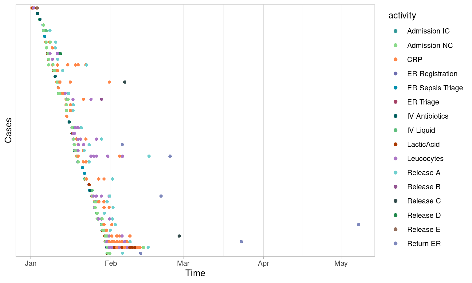
Time Period

Filtering cases by time period can be done using the filter_time_period() introduced above. There are four different filter_method’s that act as case filters:

• “start”: all cases started in an interval.
• “complete”: all cases completed in an interval.
• “contained”: all cases contained in an interval.
• “intersecting”: all cases with some activity in an interval.

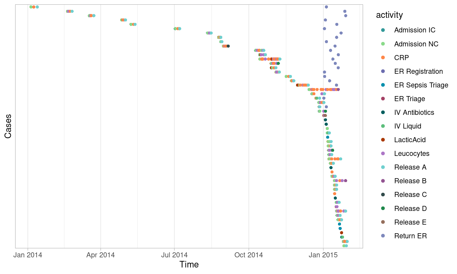
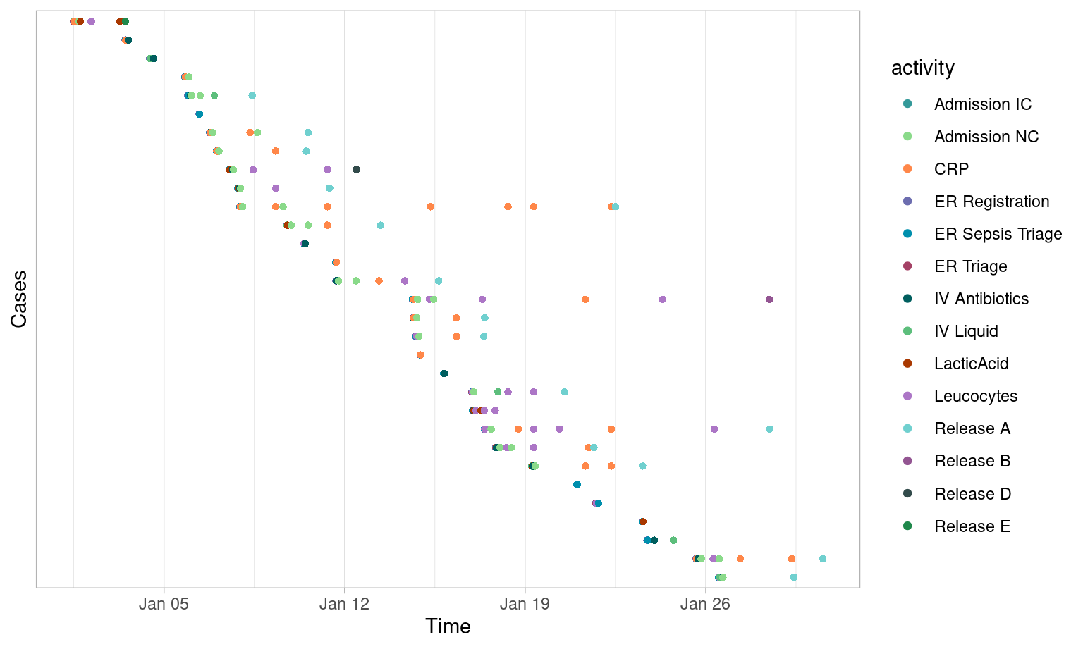
Using the same interval (the month of January 2015), you can compare the results of different filtering methods below using dotted charts.

Start

sepsis %>%
    filter_time_period(interval = ymd(c(20150101, 20150131)), filter_method = "start") %>%
    dotted_chart() 

Complete

sepsis %>%
    filter_time_period(interval = ymd(c(20150101, 20150131)), filter_method = "complete") %>%
    dotted_chart()

Contained

sepsis %>%
    filter_time_period(interval = ymd(c(20150101, 20150131)), filter_method = "contained") %>%
    dotted_chart()

Intersecting

sepsis %>%
    filter_time_period(interval = ymd(c(20150101, 20150131)), filter_method = "intersecting") %>%
    dotted_chart()

Trace Frequency

The frequency of a trace, i.e. distinct activity sequence, is the number of cases, i.e. process instances that follow this trace. filter_trace_frequency() can be used to select cases based on the amount of throughput time. There are two approaches: using an interval, or using a percentage.

Interval-based

Using filter_trace_frequency() with argument interval, you can select cases of which the trace frequency falls within a certain frequency interval. For example, all the cases from sepsis with a trace frequency between 10 and 50. traces() is used to show the changes to the log data after applying the filter.

sepsis %>%
    filter_trace_frequency(interval = c(10,50)) %>%
    traces()

## # A tibble: 5 × 3
##   trace                                    absolute_frequency relative_frequency
##   <chr>                                                 <int>              <dbl>
## 1 ER Registration,ER Triage,ER Sepsis Tri…                 35              0.333
## 2 ER Registration,ER Triage,ER Sepsis Tri…                 24              0.229
## 3 ER Registration,ER Triage,ER Sepsis Tri…                 22              0.210
## 4 ER Registration,ER Triage,ER Sepsis Tri…                 13              0.124
## 5 ER Registration,ER Triage,ER Sepsis Tri…                 11              0.105

Also here you can use half-open intervals.

sepsis %>%
    filter_trace_frequency(interval = c(5,NA)) %>%
    traces()

## # A tibble: 11 × 3
##    trace                                   absolute_frequency relative_frequency
##    <chr>                                                <int>              <dbl>
##  1 ER Registration,ER Triage,ER Sepsis Tr…                 35             0.248 
##  2 ER Registration,ER Triage,ER Sepsis Tr…                 24             0.170 
##  3 ER Registration,ER Triage,ER Sepsis Tr…                 22             0.156 
##  4 ER Registration,ER Triage,ER Sepsis Tr…                 13             0.0922
##  5 ER Registration,ER Triage,ER Sepsis Tr…                 11             0.0780
##  6 ER Registration,ER Triage,ER Sepsis Tr…                  9             0.0638
##  7 ER Registration,ER Triage,ER Sepsis Tr…                  7             0.0496
##  8 ER Registration,ER Triage,ER Sepsis Tr…                  5             0.0355
##  9 ER Registration,ER Triage,ER Sepsis Tr…                  5             0.0355
## 10 ER Registration,ER Triage,ER Sepsis Tr…                  5             0.0355
## 11 ER Registration,ER Triage,CRP,Leucocyt…                  5             0.0355

And use reverse = TRUE.

sepsis %>%
    filter_trace_frequency(interval = c(5,NA), reverse = TRUE) %>%
    traces()

## # A tibble: 835 × 3
##    trace                                   absolute_frequency relative_frequency
##    <chr>                                                <int>              <dbl>
##  1 ER Registration,ER Triage,ER Sepsis Tr…                  4            0.00440
##  2 ER Registration,ER Triage,ER Sepsis Tr…                  4            0.00440
##  3 ER Registration,ER Triage,ER Sepsis Tr…                  4            0.00440
##  4 ER Registration,ER Triage,ER Sepsis Tr…                  4            0.00440
##  5 ER Registration,ER Triage,Leucocytes,C…                  4            0.00440
##  6 ER Registration,ER Triage,ER Sepsis Tr…                  4            0.00440
##  7 ER Registration,ER Triage,ER Sepsis Tr…                  4            0.00440
##  8 ER Registration,ER Triage,ER Sepsis Tr…                  3            0.00330
##  9 ER Registration,ER Triage,LacticAcid,L…                  3            0.00330
## 10 ER Registration,ER Triage,CRP,LacticAc…                  3            0.00330
## # ℹ 825 more rows

Percentage-based

Using filter_trace_frequency() with argument percentage, you can give priority to cases with a frequent trace. For example, setting percentage = 0.2 will select at least 20% of the cases, starting with those that have the highest frequency.

sepsis %>%
    filter_trace_frequency(percentage = 0.8) %>%
    traces()

## # A tibble: 846 × 3
##    trace                                   absolute_frequency relative_frequency
##    <chr>                                                <int>              <dbl>
##  1 ER Registration,ER Triage,ER Sepsis Tr…                 35            0.0333 
##  2 ER Registration,ER Triage,ER Sepsis Tr…                 24            0.0229 
##  3 ER Registration,ER Triage,ER Sepsis Tr…                 22            0.0210 
##  4 ER Registration,ER Triage,ER Sepsis Tr…                 13            0.0124 
##  5 ER Registration,ER Triage,ER Sepsis Tr…                 11            0.0105 
##  6 ER Registration,ER Triage,ER Sepsis Tr…                  9            0.00857
##  7 ER Registration,ER Triage,ER Sepsis Tr…                  7            0.00667
##  8 ER Registration,ER Triage,ER Sepsis Tr…                  5            0.00476
##  9 ER Registration,ER Triage,ER Sepsis Tr…                  5            0.00476
## 10 ER Registration,ER Triage,ER Sepsis Tr…                  5            0.00476
## # ℹ 836 more rows

You can again set reverse = TRUE if you instead want 80% of the cases with the lowest frequency.

sepsis %>%
    filter_trace_frequency(percentage = 0.2, reverse = TRUE) %>%
    traces()

## # A tibble: 784 × 3
##    trace                                   absolute_frequency relative_frequency
##    <chr>                                                <int>              <dbl>
##  1 ER Registration,ER Triage,ER Sepsis Tr…                  1            0.00128
##  2 ER Registration,ER Triage,ER Sepsis Tr…                  1            0.00128
##  3 ER Registration,ER Triage,ER Sepsis Tr…                  1            0.00128
##  4 ER Registration,ER Triage,ER Sepsis Tr…                  1            0.00128
##  5 ER Registration,IV Liquid,ER Triage,Le…                  1            0.00128
##  6 ER Registration,ER Triage,ER Sepsis Tr…                  1            0.00128
##  7 ER Registration,ER Triage,ER Sepsis Tr…                  1            0.00128
##  8 ER Registration,ER Triage,CRP,LacticAc…                  1            0.00128
##  9 ER Registration,ER Triage,ER Sepsis Tr…                  1            0.00128
## 10 ER Registration,ER Triage,Leucocytes,C…                  1            0.00128
## # ℹ 774 more rows

Note that the obtained percentage of cases will not always be exactly the specified percentage, as there can be ties. For example, in the sepsis data set, 784 of the 1050 cases (75%) follow a distinct activity sequence. As bupaR will not break ties randomly, it will select all cases once the percentage set is higher then ca. 24%, as it will include all unique cases then still remaining in the log to get to this coverage.

Trace Length

The length of a trace, i.e. distinct activity sequence, is the number of activity instances it contains. Note that this is not necessarily equal to the number of events.

filter_trace_length() can be used to select cases based on the amount of throughput time. There are two approaches: using an interval, or using a percentage.

Interval-based

Using filter_trace_length() with argument interval, you can select cases of which the trace length falls within a certain interval. For example, all the cases of sepsis with a trace length between 10 and 50. Changes are illustrated with traces().

sepsis %>%
    filter_trace_length(interval = c(10,50)) %>%
    traces()

## # A tibble: 703 × 3
##    trace                                   absolute_frequency relative_frequency
##    <chr>                                                <int>              <dbl>
##  1 ER Registration,ER Triage,ER Sepsis Tr…                  4            0.00540
##  2 ER Registration,ER Triage,ER Sepsis Tr…                  4            0.00540
##  3 ER Registration,ER Triage,ER Sepsis Tr…                  4            0.00540
##  4 ER Registration,ER Triage,ER Sepsis Tr…                  3            0.00405
##  5 ER Registration,ER Triage,ER Sepsis Tr…                  3            0.00405
##  6 ER Registration,ER Triage,ER Sepsis Tr…                  3            0.00405
##  7 ER Registration,ER Triage,ER Sepsis Tr…                  3            0.00405
##  8 ER Registration,ER Triage,ER Sepsis Tr…                  2            0.00270
##  9 ER Registration,ER Triage,ER Sepsis Tr…                  2            0.00270
## 10 ER Registration,ER Triage,ER Sepsis Tr…                  2            0.00270
## # ℹ 693 more rows

Also here you can use half-open intervals.

sepsis %>%
    filter_trace_length(interval = c(10,NA)) %>%
    traces()

## # A tibble: 715 × 3
##    trace                                   absolute_frequency relative_frequency
##    <chr>                                                <int>              <dbl>
##  1 ER Registration,ER Triage,ER Sepsis Tr…                  4            0.00531
##  2 ER Registration,ER Triage,ER Sepsis Tr…                  4            0.00531
##  3 ER Registration,ER Triage,ER Sepsis Tr…                  4            0.00531
##  4 ER Registration,ER Triage,ER Sepsis Tr…                  3            0.00398
##  5 ER Registration,ER Triage,ER Sepsis Tr…                  3            0.00398
##  6 ER Registration,ER Triage,ER Sepsis Tr…                  3            0.00398
##  7 ER Registration,ER Triage,ER Sepsis Tr…                  3            0.00398
##  8 ER Registration,ER Triage,ER Sepsis Tr…                  2            0.00266
##  9 ER Registration,ER Triage,ER Sepsis Tr…                  2            0.00266
## 10 ER Registration,ER Triage,ER Sepsis Tr…                  2            0.00266
## # ℹ 705 more rows

And use reverse = TRUE.

sepsis %>%
    filter_trace_length(interval = c(10,NA), reverse = TRUE) %>%
    traces()

## # A tibble: 131 × 3
##    trace                                   absolute_frequency relative_frequency
##    <chr>                                                <int>              <dbl>
##  1 ER Registration,ER Triage,ER Sepsis Tr…                 35             0.118 
##  2 ER Registration,ER Triage,ER Sepsis Tr…                 24             0.0808
##  3 ER Registration,ER Triage,ER Sepsis Tr…                 22             0.0741
##  4 ER Registration,ER Triage,ER Sepsis Tr…                 13             0.0438
##  5 ER Registration,ER Triage,ER Sepsis Tr…                 11             0.0370
##  6 ER Registration,ER Triage,ER Sepsis Tr…                  9             0.0303
##  7 ER Registration,ER Triage,ER Sepsis Tr…                  7             0.0236
##  8 ER Registration,ER Triage,ER Sepsis Tr…                  5             0.0168
##  9 ER Registration,ER Triage,ER Sepsis Tr…                  5             0.0168
## 10 ER Registration,ER Triage,ER Sepsis Tr…                  5             0.0168
## # ℹ 121 more rows

Percentage-based

Using filter_trace_length() with argument percentage, you can give priority to cases with the longest length. For example, setting percentage = 0.5 will select 50% of the cases, starting with those that have the highest length. Again, changes are illustrated with traces().

sepsis %>%
    filter_trace_length(percentage = 0.5) %>%
    traces()

## # A tibble: 514 × 3
##    trace                                   absolute_frequency relative_frequency
##    <chr>                                                <int>              <dbl>
##  1 ER Registration,ER Triage,ER Sepsis Tr…                  2            0.00381
##  2 ER Registration,ER Triage,ER Sepsis Tr…                  2            0.00381
##  3 ER Registration,ER Triage,ER Sepsis Tr…                  2            0.00381
##  4 ER Registration,ER Triage,ER Sepsis Tr…                  2            0.00381
##  5 ER Registration,ER Triage,ER Sepsis Tr…                  2            0.00381
##  6 ER Registration,ER Triage,ER Sepsis Tr…                  2            0.00381
##  7 ER Registration,ER Triage,ER Sepsis Tr…                  2            0.00381
##  8 ER Registration,ER Triage,ER Sepsis Tr…                  2            0.00381
##  9 ER Registration,ER Triage,ER Sepsis Tr…                  2            0.00381
## 10 ER Registration,ER Triage,ER Sepsis Tr…                  2            0.00381
## # ℹ 504 more rows

You can again set reverse = TRUE if you instead want 50% of the cases with the lowest frequency.

sepsis %>%
    filter_trace_length(percentage = 0.5, reverse = TRUE) %>%
    traces()

## # A tibble: 337 × 3
##    trace                                   absolute_frequency relative_frequency
##    <chr>                                                <int>              <dbl>
##  1 ER Registration,ER Triage,ER Sepsis Tr…                 35            0.0667 
##  2 ER Registration,ER Triage,ER Sepsis Tr…                 24            0.0457 
##  3 ER Registration,ER Triage,ER Sepsis Tr…                 22            0.0419 
##  4 ER Registration,ER Triage,ER Sepsis Tr…                 13            0.0248 
##  5 ER Registration,ER Triage,ER Sepsis Tr…                 11            0.0210 
##  6 ER Registration,ER Triage,ER Sepsis Tr…                  9            0.0171 
##  7 ER Registration,ER Triage,ER Sepsis Tr…                  7            0.0133 
##  8 ER Registration,ER Triage,ER Sepsis Tr…                  5            0.00952
##  9 ER Registration,ER Triage,ER Sepsis Tr…                  5            0.00952
## 10 ER Registration,ER Triage,ER Sepsis Tr…                  5            0.00952
## # ℹ 327 more rows

Note that the obtained percentage of cases will not always be exactly the specified percentage, as there can be ties.

---

Read more:

Wrangling Case Filters Event Filters Generic Filtering Augment Mutate Collapse Unite

---

Copyright © 2023 bupaR - Hasselt University