bupaR Docs | Multi-dimensional analysis
![]()
Multi-dimensional analysis
By combining metrics with group_by() and augment(), you can perform analysis
that combine multiple perspectives.
For example, let’s say we want to compare throughput time (performance) with trace length (control-flow). We start by computing the throughput time per case.
##   case_id throughput_time
## 1   A1280  279.4286 weeks
## 2  A10495  247.4286 weeks
## 3  A11065  246.1429 weeks
## 4  A10981  245.0000 weeks
## 5  A11587  244.1429 weeks
## 6  A11475  244.0000 weeks
Subsequently, we add this information to the log using
augment(), and store the result as tmp.
traffic_fines %>%
    throughput_time(level = "case", units = "weeks") %>%
    augment(traffic_fines) -> tmp
Now, we have 2 options. Option 1 is to calculate the
trace_length() as well, and adding it again to the log.
We then have both the performance and coverage information in the log, and can visualize their relationship.
library(ggplot2)
tmp2 %>%
    ggplot(aes(length_absolute, throughput_time)) +
    geom_boxplot(aes(group = length_absolute))
## Don't know how to automatically pick scale for object of type <difftime>.
## Defaulting to continuous.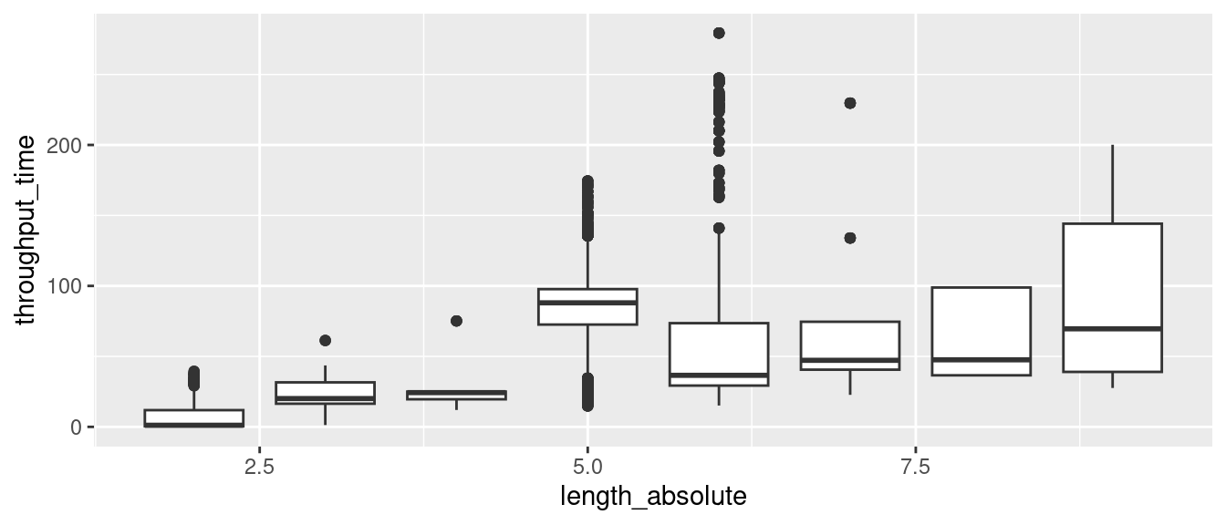 However, this requires that we have some knowledge about
ggplot2. Alternatively, we can use group_by()
and the default plot() method provided by
bupaR.
Going back to tmp, recall we have the continuous
throughput_time variable. Let’s use cut() to
create multiple categories of throughput time. We start by looking at
the throughput time distribution.
## # A tibble: 1 × 8
##   min     q1      median         mean           q3            max   st_dev iqr
##   <drtn>  <drtn>  <drtn>         <drtn>         <drtn>        <drt>  <dbl> <drt>
## 1 0 weeks 1 weeks 17.85714 weeks 42.30501 weeks 85.14286 wee… 279.…   44.8 84.1…
Let’s say use Q1, Q3 and the median to create 4 groups.
tmp %>%
    mutate(throughput_time_bin = cut(as.numeric(throughput_time), breaks = c(-Inf, 1, 17.85, 85.14, Inf)))
## # Log of 34724 events consisting of:
## 44 traces
## 10000 cases
## 34724 instances of 11 activities
## 16 resources
## Events occurred from 2006-06-17 until 2012-03-26
##
## # Variables were mapped as follows:
## Case identifier: case_id
## Activity identifier: activity
## Resource identifier: resource
## Activity instance identifier: activity_instance_id
## Timestamp: timestamp
## Lifecycle transition: lifecycle
##
## # A tibble: 34,724 × 20
## case_id activity lifecycle resource timestamp amount article
## <chr> <fct> <fct> <fct> <dttm> <chr> <dbl>
## 1 A1 Create Fine complete 561 2006-07-24 00:00:00 35.0 157
## 2 A1 Send Fine complete <NA> 2006-12-05 00:00:00 <NA> NA
## 3 A100 Create Fine complete 561 2006-08-02 00:00:00 35.0 157
## 4 A100 Send Fine complete <NA> 2006-12-12 00:00:00 <NA> NA
## 5 A100 Insert Fine No… complete <NA> 2007-01-15 00:00:00 <NA> NA
## 6 A100 Add penalty complete <NA> 2007-03-16 00:00:00 71.5 NA
## 7 A100 Send for Credi… complete <NA> 2009-03-30 00:00:00 <NA> NA
## 8 A10000 Create Fine complete 561 2007-03-09 00:00:00 36.0 157
## 9 A10000 Send Fine complete <NA> 2007-07-17 00:00:00 <NA> NA
## 10 A10000 Insert Fine No… complete <NA> 2007-08-02 00:00:00 <NA> NA
## # ℹ 34,714 more rows
## # ℹ 13 more variables: dismissal <chr>, expense <chr>, lastsent <chr>,
## # matricola <dbl>, notificationtype <chr>, paymentamount <dbl>, points <dbl>,
## # totalpaymentamount <chr>, vehicleclass <chr>, activity_instance_id <chr>,
## # .order <int>, throughput_time <drtn>, throughput_time_bin <fct>Observe that we have now 4 groups under throughput_time_bin with the roughly same number of cases.
tmp %>%
    mutate(throughput_time_bin = cut(as.numeric(throughput_time), breaks = c(-Inf, 1, 17.85, 85.14, Inf))) %>%
    group_by(throughput_time_bin) %>%
    n_cases()
## # A tibble: 4 × 2
## throughput_time_bin n_cases
## <fct> <int>
## 1 (-Inf,1] 2567
## 2 (1,17.9] 2428
## 3 (17.9,85.1] 2484
## 4 (85.1, Inf] 2521Now, instead of using group_by() and
n_cases(), we can use group_by() followed by
trace_length(). This gives us the distribution of the trace
length, for each of the groups.
tmp %>%
    mutate(throughput_time_bin = cut(as.numeric(throughput_time), breaks = c(-Inf, 1, 17.85, 85.14, Inf))) %>%
    group_by(throughput_time_bin) %>%
    trace_length()
## # A tibble: 4 × 9
## throughput_time_bin min q1 median mean q3 max st_dev iqr
## <fct> <int> <dbl> <dbl> <dbl> <dbl> <int> <dbl> <dbl>
## 1 (-Inf,1] 2 2 2 2 2 2 0 0
## 2 (1,17.9] 2 2 2 2.02 2 6 0.237 0
## 3 (17.9,85.1] 2 5 5 4.78 5 9 1.28 0
## 4 (85.1, Inf] 5 5 5 5.08 5 9 0.417 0We plot this new information:
tmp %>%
mutate(throughput_time_bin = cut(as.numeric(throughput_time), breaks = c(-Inf, 1, 17.85, 85.14, Inf))) %>%
group_by(throughput_time_bin) %>%
trace_length() %>%
plot()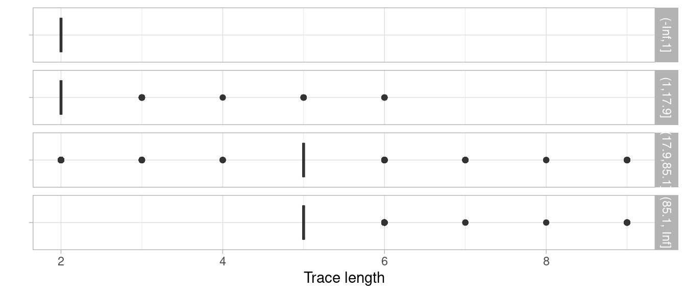 While the resulting default plot might not be ideal for your situation
(as here, it doesn’t work well with trace lengths discrete
characteristic), you can get a first insight without needing any
additional visualization expertise.
While the resulting default plot might not be ideal for your situation
(as here, it doesn’t work well with trace lengths discrete
characteristic), you can get a first insight without needing any
additional visualization expertise.
Note that, if we turn the analysis the other way around (e.g. what is
the impact of trace length on throughput time?), things get even easier
as the discrete trace length variable can be directly fed to
group_by().
traffic_fines %>%
    trace_length(level = "case") %>%
    augment(traffic_fines, prefix = "length") %>%
    group_by(length_absolute) %>%
    throughput_time() %>%
    plot()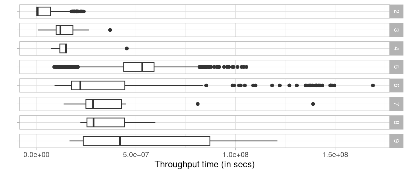
Finally, note that you are not restricted to combining calculated metrics. You can also combine metrics with data attributes.
## # A tibble: 43 × 9
##    group                      min    q1 median  mean    q3   max st_dev   iqr
##    <fct>                    <int> <dbl>  <dbl> <dbl> <dbl> <int>  <dbl> <dbl>
##  1 Anesthesiology               1     1      1  1.12  1        2  0.354  0
##  2 Anesthesiology clinic        1     1      1  1.03  1        2  0.174  0
##  3 Cardiology clinic            3     3      3  3     3        3 NA      0
##  4 Cardiovascular clinics       1     1      1  1.88  2        8  1.31   1
##  5 Clinical Neurophysiology     1     1      1  1     1        1 NA      0
##  6 Day Centre - treatment       1     1      2  1.76  2        3  0.577  1
##  7 Day Centre - ward            1     2      2  1.93  2        4  0.521  0
##  8 Diet Studies                 1     1      1  2.12  2       18  2.25   1
##  9 Emergency room               1     1      1  1.5   1.75     3  0.837  0.75
## 10 Endoscopy                    1     1      2  2.27  3        5  1.42   2
## # ℹ 33 more rows
Copyright © 2025 bupaR - Hasselt University